3D Views - Planes and Relief Surfaces
- ian macleod (Deactivated)
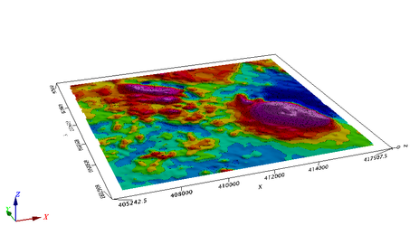
Draw to a Flat Plane in 3D
In this first lesson we will simply draw to the default drawing plane on a new 3D view.
import geosoft.gxpy.gx as gx
import geosoft.gxpy.view as gxview
import geosoft.gxpy.group as gxgroup
import geosoft.gxpy.agg as gxagg
import geosoft.gxpy.grid as gxgrd
import geosoft.gxpy.viewer as gxviewer

gxc = gx.GXpy()

grid_file = 'Wittichica Creek Residual Total Field.grd'

# create a 3D view
with gxview.View_3d.new("TMI on a plane",
                        area_2d=gxgrd.Grid(grid_file).extent_2d(),
                        coordinate_system=gxgrd.Grid(grid_file).coordinate_system,
                        overwrite=True) as v:

    v3d_name = v.file_name

    # add the grid image to the view, with shading, ands contour
    gxgroup.Aggregate_group.new(v, gxagg.Aggregate_image.new(grid_file, shade=True, contour=20))
    gxgroup.contour(v, 'TMI_contour', grid_file)


# display the map in a Geosoft viewer
gxviewer.view_document(v3d_name, wait_for_close=False)
| Line | Commentary |
|---|---|
| 13 | We create a new 3D view that will contain 3D objects. Although not necessary, we define the extent to match the grid and it is good practice to establish the spatial coordinate system. This will create a file named "TIM in relief.geosoft_3dv". A 3D group can contain 3D objects and it has a default drawing plane on which 2D objects are drawn. The initial default drawing plane is a horizontal plane at an elevation = 0. |
| 21, 22 | Create an aggregate group, which will be drawn on the default drawing plane, and add contours. |
| 26 | Open a viewer and display the new document. |
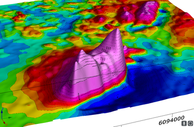
Draw on a 3D Relief Surface
In this lesson we use the data values to define a 3D relief surface for the drawing plane, which transforms from a flat plane to a function surface with function relief defined by the grid data values.
import geosoft.gxpy.gx as gx
import geosoft.gxpy.view as gxview
import geosoft.gxpy.group as gxgroup
import geosoft.gxpy.agg as gxagg
import geosoft.gxpy.grid as gxgrd
import geosoft.gxpy.viewer as gxviewer

gxc = gx.GXpy()

grid_file = 'Wittichica Creek Residual Total Field.grd'

# create a 3D view
with gxview.View_3d.new("TMI in relief",
                        area_2d=gxgrd.Grid.open(grid_file).extent_2d(),
                        coordinate_system=gxgrd.Grid.open(grid_file).coordinate_system,
                        overwrite=True) as v:

    v3d_name = v.file_name

    # use the data grid as the relief surface
    v.set_plane_relief_surface(grid_file)

    # add the grid image to the view, with shading, 20 nT contour interval to match default contour lines
    gxgroup.Aggregate_group.new(v, gxagg.Aggregate_image.new(grid_file, shade=True, contour=20))
    gxgroup.contour(v, 'TMI_contour', grid_file)


# display the map in a Geosoft viewer
gxviewer.view_document(v3d_name, wait_for_close=False)
| Line | Commentary |
|---|---|
| 21 | This gives the drawing plane a relief surface defined by data values of the grid. |
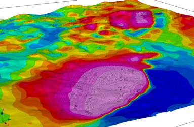
Display Data on the Digital Elevation Model
    # use the DEM as the relief surface
    v.set_plane_relief_surface('Wittichica DEM.grd')
| Line | Commentary |
|---|---|
| 21 | This is the same as the last example except that this time we use the actual DEM grid to define the relief surface. The TMI aggregate will now be draped into the DEM surface. |
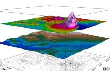
Stacked Planes
A common presentation shows different data layers appearing to float relative to each other. Here we create two floating planes shown relative to the DEM, which is shown as a relief surface at the expected Z elevation. The TMI data is shown as a relief surface floating above the DEM with relief determined by the TMI values, and a contour of the DEM data on a flat plane beneath the DEM surface.
tmi_file = 'Wittichica Creek Residual Total Field.grd'
dem_file = 'Wittichica DEM.grd'

# create a 3D view
with gxview.View_3d.new("TMI drapped on DEM",
                        area_2d=gxgrd.Grid.open(tmi_file).extent_2d(),
                        coordinate_system=gxgrd.Grid.open(tmi_file).coordinate_system,
                        scale=5000,
                        overwrite=True) as v:

    v3d_name = v.file_name

    # use the DEM as the relief surface
    v.set_plane_relief_surface(dem_file)
    gxgroup.Aggregate_group.new(v, gxagg.Aggregate_image.new(dem_file,
                                                             color_map='elevation.tbl'))

    # relief plane for the TMI, offset to elevation 2000
    v.new_drawing_plane('TMI relief')
    v.set_plane_relief_surface(tmi_file, base=-4000)
    gxgroup.Aggregate_group.new(v, gxagg.Aggregate_image.new(tmi_file))
    gxgroup.contour(v, 'TMI_contour', tmi_file)

    # add DEM contours on a plane floating beneath the DEM
    v.new_drawing_plane('Scratch plane', offset=(0, 0, -2000))
    gxgroup.contour(v, 'DEM contour', tmi_file)

# display the map in a Geosoft viewer
gxviewer.view_document(v3d_name, wait_for_close=False)
| Line | Commentary |
|---|---|
| 25 | Colour the dem surface using the 'elevation.tbl' colour table. |
| 29 | Make the base of the TMI -4000, which locates the TMI surface above the DEM surface. Note that in this case the TMI is naturally scaled to a reasonable relief surface with the default scale=1. For other data you may need to change the scale to something appropriate for the data. |
| 34 | To locate a plane in space without defining a relief surface we can define the location using the offset= parameter. In this case we are offsetting the plane z origin to be at -2000. |