For this lesson we will start with a data grid, in this case a residual total magnetic intensity (TMI) data grid for the Wittichica Creek area of British Columbia, Canada. This data was downloaded from the Geoscience Data Portal of the Geoscience Canada using Geosoft Seeker.

The most common requirement for a grid is to be able to present the data as a colour image that can be viewed or printed. In this exercise we will first view the grid, then add contours, shading and a colour legend, and finally we will add location annotations and complete the map ready for printing or sharing.

What You Will Learn

Understanding of Geosoft Maps as a container for 2D (and 3D) Views.
How to create a map with a data view and a base view.
How to display a coloured grid in a data view.
How to add contours, shading and a colour legend.
How to add coordinate annotations and annotate the base view with text.
How to save a map as an image file.

Tutorial Files

Files for this lesson are here:

https://github.com/GeosoftInc/gxpy/tree/9.3/examples/tutorial/2D%20Views%20and%20Maps

Run this script to download data:

https://github.com/GeosoftInc/gxpy/raw/9.3/examples/tutorial/2D%20Views%20and%20Maps/get_data_files.py

Jupyter Notebook

On this page

Lesson Guide

Tutorial data and code

Jupyter Notebooks

Understanding Geosoft Maps and Views

Geosoft maps are used to present geoscience information on a 2D surface, which can be a computer screen or printed on paper.

Geosoft Maps are stored in a file that has a descriptive name and an extension .map.
A Map can be thought of as a physical piece of paper, and we use map centimeters or map millimetres to reference locations relative to the bottom-left corner, which is location (0,0).
A Map contains Views, and a Map may have any number of Views.
A View represents some spatial extent within a defined Earth coordinate system that is scaled and located as desired on the surface of the map.
Views can be 2D or 3D, with 3D views rendered on a map as a 2D perspective of the information in the 3D View..
Views contain named Groups, with each Group containing a set of graphical elements that display spatial information. Basic drawing Groups contain lines, coloured areas and text. More advanced Group types support more complex data structures like Aggregates for grids and images, Voxels that display a Geosoft voxette, or a CSymb Group that contains data points coloured by size based on a data value.
3D Views can contain 3D Groups, such as a something drawn on a relief surface, or a 3D Geosoft Geosurface, or a set of vectors from a Geosoft Vector voxel.
Geosoft Maps can be opened and viewed in a Geosoft Viewer.

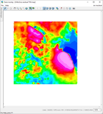
Display a grid on a map

One of the most common tasks is to display a data grid in colour:

grid_display_map.py

import geosoft.gxpy.gx as gx
import geosoft.gxpy.map as gxmap
import geosoft.gxpy.view as gxview
import geosoft.gxpy.group as gxgroup
import geosoft.gxpy.agg as gxagg
import geosoft.gxpy.grid as gxgrd
import geosoft.gxpy.viewer as gxviewer

gxc = gx.GXpy()

# create a map from the grid coordinate system and extent
with gxgrd.Grid('Wittichica Creek Residual Total Field.grd') as grd:
    grid_file_name = grd.file_name_decorated

    # create a map for this grid on A4 media, scale to fit the extent
    with gxmap.Map.new('Wittichica residual TMI',
                       data_area=grd.extent_2d(),
                       media="A4",
                       margins=(1, 3.5, 3, 1),
                       coordinate_system=grd.coordinate_system,
                       overwrite=True) as gmap:
        map_file_name = gmap.file_name

# draw into the views on the map. We are reopening the map as the Aggregate class only works with a closed grid.
with gxmap.Map.open(map_file_name) as gmap:

    # work with the data view
    with gxview.View.open(gmap, "data") as v:

        # add the grid image to the view
        with gxagg.Aggregate_image.new(grid_file_name) as agg:
            gxgroup.Aggregate_group.new(v, agg)

# display the map in a Geosoft viewer
gxviewer.view_document(map_file_name, wait_for_close=False)

Line	Commentary
12	Open the grid so we can use the grid method extent_2d() (line 17) and grid property coordinate_system (line 20).
13	We save the full decorated grid name so we can use this at line 31 to create an Aggregate image of the grid. Note that an Aggregate class instance needs access to the grid file, not just a grid instance. See the comment for line 25 below.
16	Here we create a new map, scaled to fit the extent of the grid (line 17) and fit within A4 media (line 18). We want margins around the data as we will be annotating the map a bit later, so we set (left, right, bottom, top) margins in cm at line 19.
20	The gxmap.Map.new() method will create a map with two views, a 'base' view which is scaled to map units and a 'data' view that is scaled to the units of the data_area. It is always good practice to define the coordinate system of the 'data' view, which in this case will be the same as the coordinate system of the grid.
22	We save the full path name of the created map.
25	Here we re-open the map so we can draw on it. We would be able to draw on the map in the last with... as gmap: but we need access to the grid file (not a grid instance) to create an Aggregate at line 31, so we need to exit the with ... as grd: context that was created at line 12.
31	An Aggregate instance can hold any number of grid layers, which are combined to create a single image within a view. The Aggregate class handles re-projection and resampling of images to match the first grid/image layer and provides a number of methods to manipulate image layers. In this case we only need one layer and we will accept default colouring, which applies your users default preference. This would normally be the default Geosoft colour ramp and equal-area colouring.
32	A new Aggregate_group is in the data view.
35	Display the map in the Geosoft Viewer.

Add Contours and Shading

Now we will improve the script by adding contour lines and a shading effect. We will also make a double-line outer-contour.

grid_display_map_shade_contour

import geosoft.gxpy.gx as gx
import geosoft.gxpy.map as gxmap
import geosoft.gxpy.view as gxview
import geosoft.gxpy.group as gxgroup
import geosoft.gxpy.agg as gxagg
import geosoft.gxpy.grid as gxgrd
import geosoft.gxpy.viewer as gxviewer

gxc = gx.GXpy()

# create a map from grid coordinate system and extent
with gxgrd.Grid('Wittichica Creek Residual Total Field.grd') as grd:
    grid_file_name = grd.file_name_decorated

    # create a map for this grid on A4 media, scale to fit the extent
    with gxmap.Map.new('Wittichica residual TMI',
                       data_area=grd.extent_2d(),
                       media="A4",
                       margins=(1, 3.5, 3, 1),
                       coordinate_system=grd.coordinate_system,
                       overwrite=True) as gmap:
        map_file_name = gmap.file_name

# draw into the views on the map. We are reopening the map as the Aggregate class only works with a closed grid.
with gxmap.Map.open(map_file_name) as gmap:

    # work with the data view, draw a line around the data view
    with gxview.View.open(gmap, "data") as v:

        # add the grid image to the view, with shading, 20 nT contour interval to match default contour lines
        with gxagg.Aggregate_image.new(grid_file_name, shade=True, contour=20) as agg:
            gxgroup.Aggregate_group.new(v, agg)

		# contour the grid
        gxgroup.contour(v, 'TMI_contour', grid_file_name)

# display the map in a Geosoft viewer
gxviewer.view_document(map_file_name, wait_for_close=False)

Line

Commentary

31

The shade=True will add a shading effect to the aggregate image.

The contour=20 will reduce colours and ensure that colour breaks or on an even multiple of 20 nT thus will line-up with the contours created at line 36. The contour method is currently very simple and chooses a reasonable contour interval based on the data. We in fact first had a look at the default chosen and observed that it was 20 nT, which we have specified here.

35

Draw contours from a grid, which are placed in a drawing group named "TMI_contour"

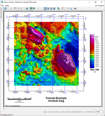
Location Reference, Scale Bar, Colour Legend and Title

Now we will improve the map my adding location reference annotations, a scale bar, colour legend and map title.

grid_shade_contour_annotate.py

import geosoft.gxpy.gx as gx
import geosoft.gxpy.map as gxmap
import geosoft.gxpy.view as gxview
import geosoft.gxpy.group as gxgroup
import geosoft.gxpy.agg as gxagg
import geosoft.gxpy.grid as gxgrd
import geosoft.gxpy.viewer as gxviewer

gxc = gx.GXpy()

# create a map from grid coordinate system and extent
with gxgrd.Grid('Wittichica Creek Residual Total Field.grd') as grd:
    grid_file_name = grd.file_name_decorated

    # create a map for this grid on A4 media, scale to fit the extent
    with gxmap.Map.new('Wittichica residual TMI',
                       data_area=grd.extent_2d(),
                       media="A4",
                       margins=(1, 3.5, 3, 1),
                       coordinate_system=grd.coordinate_system,
                       overwrite=True) as gmap:
        map_file_name = gmap.file_name

# draw into the views on the map. We are reopening the map as the Aggregate class only works with a closed grid.
with gxmap.Map.open(map_file_name) as gmap:

    # work with the data view, draw a line around the data view
    with gxview.View.open(gmap, "data") as v:

        # add the grid image to the view, with shading, 20 nT contour interval to match default contour lines
        with gxagg.Aggregate_image.new(grid_file_name, shade=True, contour=20) as agg:
            gxgroup.Aggregate_group.new(v, agg)

            # colour legend
            gxgroup.legend_color_bar(v, 'TMI_legend',
                                     title='Res TMI\nnT',
                                     location=(1.2,0),
                                     cmap=agg.layer_color_map(0),
                                     cmap2=agg.layer_color_map(1))

        # contour the grid
        gxgroup.contour(v, 'TMI_contour', grid_file_name)

    # map title and creator tag
    with gxview.View.open(gmap, "base") as v:
        with gxgroup.Draw(v, 'title') as g:

            g.text("Tutorial Example\nresidual mag",
                   reference=gxgroup.REF_BOTTOM_CENTER,
                   location=(100, 10),
                   text_def=gxgroup.Text_def(height=3.5,
                                             weight=gxgroup.FONT_WEIGHT_BOLD))
            g.text("created by:" + gxc.gid,
                   location=(1, 1.5),
                   text_def=gxgroup.Text_def(height=1.2,
                                             italics=True))

    # add a map surround to the map
    gmap.surround(outer_pen='kt500', inner_pen='kt100', gap=0.1)

    # annotate the data view locations
    gmap.annotate_data_xy(grid=gxmap.GRID_CROSSES)
    gmap.annotate_data_ll(grid=gxmap.GRID_LINES,
                          grid_pen=gxgroup.Pen(line_color='b'),
                          text_def=gxgroup.Text_def(color='b',
                                                    height=0.15,
                                                    italics=True))
    # scale bar
    gmap.scale_bar(location=(1, 3, 1.5),
                   text_def=gxgroup.Text_def(height=0.15))

# display the map in a Geosoft viewer
gxviewer.view_document(map_file_name, wait_for_close=False)

Line	Commentary
35	The legend_color_bar() function creates a colour bar from one or two Color_map instances, which are identified by the cmap= and cmap2= arguments. The Aggregate layers each have a Color_map instance which is accessed using the layer_color_map method of the aggregate. The first layer will be used as the main labelled bar and the second layer will be blended horizontally through each colour in order to show the shaded effect.
45	We open the base view so we can add some text for the title. It is always a nice touch to identify the person who created the map, which we do at line 53.
49	Center the text by positioning the bottom-center of the text box at the location=(100, 10). The 'base' view is scaled in mm for the purpose of drawing, and here we locate the text at (100, 10) mm from the bottom left corner of the 'base' view, which is also the origin of the map..
59	The geosoft.gxpy.map module has a number of general-purpose functions that can be used to finish details on a map. The surround() function draws neat-lines around the edge of the map. In this example we define pens using the Geosoft mapplot string format "kt500" and "kt100", "k" indicating black, and "t500" indicating the the thickness in microns (see Pen.from_mapplot_string()), One could also create a Pen instance as is used elsewhere.
62	The annotate_data_xy() method adds coordinate annotations to the edge of the current 'data' view.
63	The annotate_data_ll() method adds longitude and latitude coordinate annotations to the edge of the current 'data' view. Longitude and Latitude reference lines are determined based on the coordinate system of the 'data' view, which must be defined for this to work.
69	Add a map scale bar.

Save Map as an Image File

Maps can be saved as image files in a number of formats. This can be useful to produce high-quality images to be included in reports or other graphical applications.

To do this use the geosoft.gxpy.map.save_as_image() function, which can be added to the end of the last program script, This will create a default 1000 pixel-wide image, though the desired image size can be adjusted using the pix_width= or pix_height= function arguments.

# save to a PNG file
gxmap.save_as_image(map_file_name, "wittichica_mag.png", type=gxmap.RASTER_FORMAT_PNG)

GX Developer 9.3

2D Views and Maps